Introduction
This vignette compares joint modeling (JSM package) with time-varying Cox regression using simulated data with known parameters. Joint models properly account for measurement error and informative dropout, while naive approaches may yield biased estimates.
Setup
library(JointODE)
library(JSM)
library(nlme)
library(survival)
library(ggplot2)
library(dplyr)
library(tidyr)
library(patchwork)

set.seed(2024)
# Generate data with known parameters
sim_data <- JointODE::simulate(
  n = 400, # Number of subjects
  sigma_b = 0.1, # Measurement error SD
  verbose = FALSE
)

long_data <- sim_data$longitudinal_data
surv_data <- sim_data$survival_data

# Data summary
cat(sprintf(
  "Dataset: %d subjects, %d observations\n",
  n_distinct(long_data$id), nrow(long_data)
))
#> Dataset: 400 subjects, 5468 observations
cat(sprintf(
  "Events: %.0f%% (median follow-up: %.1f)\n",
  100 * mean(surv_data$status),
  median(surv_data$time)
))
#> Events: 74% (median follow-up: 5.3)
Data Preparation
# Format data for JSM package
jsm_data <- dataPreprocess(
  long = long_data %>% rename(ID = id),
  surv = surv_data %>% rename(ID = id, survtime = time),
  id.col = "ID",
  long.time.col = "time",
  surv.time.col = "survtime",
  surv.event.col = "status"
) %>%
  rename(
    obstime = time,
    start = start.join,
    stop = stop.join,
    event = event.join
  )

surv_data_jsm <- surv_data %>% rename(ID = id, survtime = time)
Exploratory Analysis
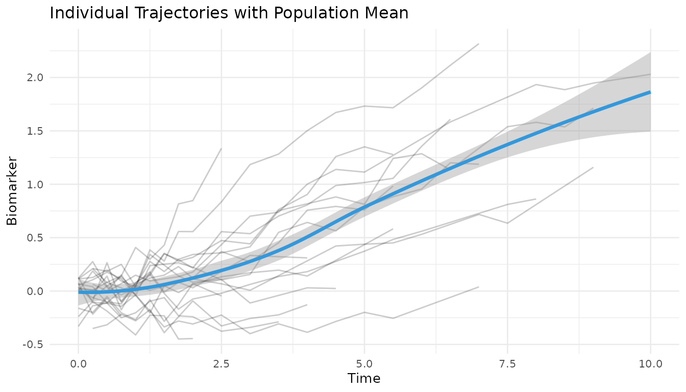
# Visualize longitudinal trajectories
long_data %>%
  filter(id %in% sample(unique(id), 20)) %>%
  ggplot(aes(time, v)) +
  geom_line(aes(group = id), alpha = 0.2) +
  geom_smooth(se = TRUE, color = "#3498DB", linewidth = 1.2) +
  theme_minimal(base_size = 10) +
  labs(
    x = "Time", y = "Biomarker",
    title = "Individual Trajectories with Population Mean"
  )
# Survival distribution
km_fit <- survfit(Surv(survtime, status) ~ 1, data = surv_data_jsm)
plot(km_fit,
  xlab = "Time", ylab = "Survival Probability",
  main = sprintf(
    "Event Rate: %.0f%%, Median: %.1f",
    100 * mean(surv_data_jsm$status), median(km_fit)
  ),
  conf.int = TRUE, mark.time = FALSE, lwd = 2, col = "#E74C3C"
)
grid(lty = 3, col = "gray90")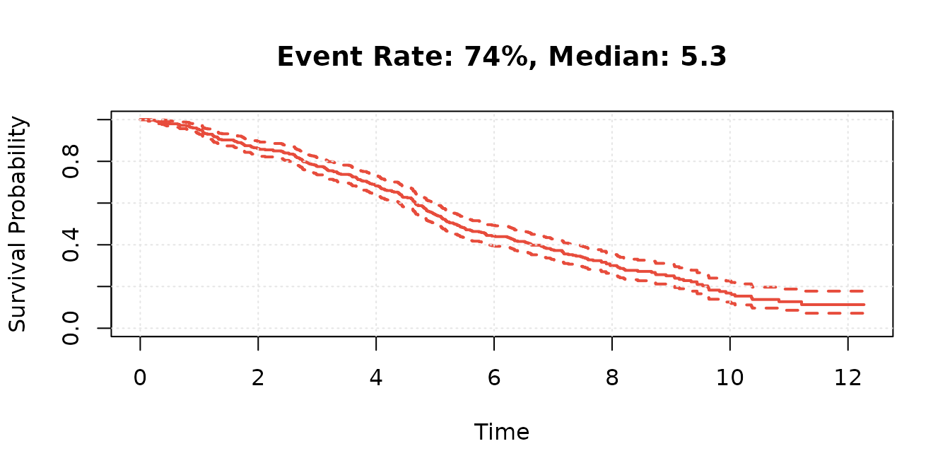
Model Fitting
Longitudinal Model
fit_lme <- lme(
  v ~ obstime + x1 + x2,
  random = ~ 1 | ID,
  data = jsm_data,
  control = lmeControl(opt = "optim")
)

summary(fit_lme)
#> Linear mixed-effects model fit by REML
#>   Data: jsm_data
#>        AIC      BIC    logLik
#>   3858.946 3898.581 -1923.473
#>
#> Random effects:
#>  Formula: ~1 | ID
#>         (Intercept)  Residual
#> StdDev:   0.1537356 0.3266545
#>
#> Fixed effects:  v ~ obstime + x1 + x2
#>                   Value   Std.Error   DF  t-value p-value
#> (Intercept) -0.09442697 0.010262856 5067 -9.20085       0
#> obstime      0.09609937 0.002036320 5067 47.19266       0
#> x1           0.29023869 0.009439471  397 30.74735       0
#> x2           0.14462882 0.009086661  397 15.91661       0
#>  Correlation:
#>         (Intr) obstim x1
#> obstime -0.467
#> x1       0.017  0.068
#> x2      -0.037  0.028 -0.079
#>
#> Standardized Within-Group Residuals:
#>         Min          Q1         Med          Q3         Max
#> -3.71628471 -0.56266263 -0.06583742  0.50977566  5.17633036
#>
#> Number of Observations: 5468
#> Number of Groups: 400
Baseline Survival
fit_cox <- coxph(
  Surv(start, stop, event) ~ w1 + w2,
  data = jsm_data,
  x = TRUE
)
summary(fit_cox)
#> Call:
#> coxph(formula = Surv(start, stop, event) ~ w1 + w2, data = jsm_data,
#>     x = TRUE)
#>
#>   n= 5468, number of events= 294
#>
#>        coef exp(coef) se(coef)      z Pr(>|z|)
#> w1  0.31642   1.37221  0.06201  5.103 3.35e-07 ***
#> w2 -0.12467   0.88279  0.05513 -2.262   0.0237 *
#> ---
#> Signif. codes:  0 '***' 0.001 '**' 0.01 '*' 0.05 '.' 0.1 ' ' 1
#>
#>    exp(coef) exp(-coef) lower .95 upper .95
#> w1    1.3722     0.7288    1.2152    1.5495
#> w2    0.8828     1.1328    0.7924    0.9835
#>
#> Concordance= 0.596  (se = 0.018 )
#> Likelihood ratio test= 31.33  on 2 df,   p=2e-07
#> Wald test            = 31.06  on 2 df,   p=2e-07
#> Score (logrank) test = 31  on 2 df,   p=2e-07
Joint Model
fit_jsm <- jmodelTM(
  fit_lme,
  fit_cox,
  data = jsm_data,
  timeVarY = "obstime",
  control = list(
    delta = 1e-8,
    max.iter = 500,
    tol.P = 1e-04
  )
)
#> Running jmodelTM(), may take some time to finish.

summary(fit_jsm)
#>
#> Call:
#> jmodelTM(fitLME = fit_lme, fitCOX = fit_cox, data = jsm_data,
#>     timeVarY = "obstime", control = list(delta = 1e-08, max.iter = 500,
#>         tol.P = 1e-04))
#>
#> Data Descriptives:
#> Longitudinal Process     Survival Process
#> Number of Observations: 5468 Number of Events: 294 (73.5%)
#> Number of Groups: 400
#>      AIC      BIC    logLik
#>  7477.29 7513.213 -3729.645
#>
#> Coefficients:
#> Longitudinal Process: Linear mixed-effects model
#>               Estimate     StdErr z.value   p.value
#> (Intercept) -0.0949470  0.0101934 -9.3146 < 2.2e-16 ***
#> obstime      0.0968450  0.0020406 47.4581 < 2.2e-16 ***
#> x1           0.2911387  0.0094537 30.7962 < 2.2e-16 ***
#> x2           0.1448967  0.0090177 16.0681 < 2.2e-16 ***
#> ---
#> Signif. codes:  0 '***' 0.001 '**' 0.01 '*' 0.05 '.' 0.1 ' ' 1
#>
#> Survival Process: Proportional hazards model with unspecified baseline hazard function
#>     Estimate    StdErr z.value   p.value
#> w1  0.327666  0.062444  5.2473 1.543e-07 ***
#> w2 -0.149429  0.055723 -2.6817  0.007326 **
#> v   0.810758  0.157135  5.1596 2.474e-07 ***
#> ---
#> Signif. codes:  0 '***' 0.001 '**' 0.01 '*' 0.05 '.' 0.1 ' ' 1
#>
#> Variance Components:
#>             StdDev
#> Random   0.1518726
#> Residual 0.3267628
#>
#> Integration: (Adaptive Gauss-Hermite Quadrature)
#> quadrature points: 9
#>
#> StdErr Estimation:
#> method: profile Fisher score with Richardson extrapolation
#>
#> Optimization:
#> convergence: success
#> iterations: 6
Time-Varying Cox
fit_tvcox <- coxph(
  Surv(start, stop, event) ~ w1 + w2 + v + cluster(ID),
  data = jsm_data
)

summary(fit_tvcox)
#> Call:
#> coxph(formula = Surv(start, stop, event) ~ w1 + w2 + v, data = jsm_data,
#>     cluster = ID)
#>
#>   n= 5468, number of events= 294
#>
#>        coef exp(coef) se(coef) robust se      z Pr(>|z|)
#> w1  0.32673   1.38642  0.06235   0.06226  5.248 1.54e-07 ***
#> w2 -0.15695   0.85475  0.05573   0.05411 -2.900  0.00373 **
#> v   0.62340   1.86526  0.09189   0.08631  7.222 5.11e-13 ***
#> ---
#> Signif. codes:  0 '***' 0.001 '**' 0.01 '*' 0.05 '.' 0.1 ' ' 1
#>
#>    exp(coef) exp(-coef) lower .95 upper .95
#> w1    1.3864     0.7213    1.2271    1.5664
#> w2    0.8547     1.1699    0.7687    0.9504
#> v     1.8653     0.5361    1.5750    2.2091
#>
#> Concordance= 0.64  (se = 0.017 )
#> Likelihood ratio test= 77.8  on 3 df,   p=<2e-16
#> Wald test            = 83.18  on 3 df,   p=<2e-16
#> Score (logrank) test = 74.57  on 3 df,   p=4e-16,   Robust = 67.83  p=1e-14
#>
#>   (Note: the likelihood ratio and score tests assume independence of
#>      observations within a cluster, the Wald and robust score tests do not).
Comparison
# True parameter values (using defaults from JointODE::simulate)
# alpha[1] = 0.3 (value effect), phi = c(0.2, -0.15) for survival covariates
true_params <- data.frame(
  param = c("Association", "w1", "w2"),
  true_value = c(0.5, 0.2, -0.15)
)

# Extract and organize coefficients
extract_coef <- function(jsm, tvcox) {
  jsm_vcov <- sqrt(diag(jsm$Vcov))
  tvcox_summ <- summary(tvcox)$coefficients

  data.frame(
    param = c("Association", "w1", "w2"),
    jsm_est = c(
      jsm$coefficients$alpha,
      jsm$coefficients$phi[c("w1", "w2")]
    ),
    jsm_se = c(
      jsm_vcov["alpha:v"],
      jsm_vcov[c("phi:w1", "phi:w2")]
    ),
    tvc_est = coef(tvcox)[c("v", "w1", "w2")],
    tvc_se = tvcox_summ[c("v", "w1", "w2"), "se(coef)"]
  ) %>%
    mutate(across(c("jsm_est", "jsm_se", "tvc_est", "tvc_se"), as.numeric))
}

comp <- extract_coef(fit_jsm, fit_tvcox) %>%
  left_join(true_params, by = "param") %>%
  mutate(
    diff = jsm_est - tvc_est,
    diff_pct = 100 * diff / abs(tvc_est),
    jsm_p = 2 * pnorm(-abs(jsm_est / jsm_se)),
    tvc_p = 2 * pnorm(-abs(tvc_est / tvc_se)),
    jsm_bias = jsm_est - true_value,
    tvc_bias = tvc_est - true_value
  )

# Summary table with significance stars
format_est <- function(est, se, p) {
  stars <- dplyr::case_when(
    p < 0.001 ~ "***",
    p < 0.01 ~ "**",
    p < 0.05 ~ "*",
    TRUE ~ ""
  )
  sprintf("%.3f (%.3f)%s", est, se, stars)
}

# Simple comparison table
comp %>%
  mutate(
    Parameter = c("α (Association)", "β₁ (w1)", "β₂ (w2)"),
    True = sprintf("%.2f", true_value),
    `JSM` = format_est(jsm_est, jsm_se, jsm_p),
    `TVC` = format_est(tvc_est, tvc_se, tvc_p),
    `JSM Bias` = sprintf("%+.3f", jsm_bias),
    `TVC Bias` = sprintf("%+.3f", tvc_bias)
  ) %>%
  select(Parameter, True, JSM, TVC, `JSM Bias`, `TVC Bias`) %>%
  knitr::kable(
    caption = "Parameter Estimates (* p<0.05, ** p<0.01, *** p<0.001)",
    align = c("l", rep("c", 5))
)| Parameter | True | JSM | TVC | JSM Bias | TVC Bias |
|---|---|---|---|---|---|
| α (Association) | 0.50 | 0.811 (0.157)*** | 0.623 (0.092)*** | +0.311 | +0.123 |
| β₁ (w1) | 0.20 | 0.328 (0.062)*** | 0.327 (0.062)*** | +0.128 | +0.127 |
| β₂ (w2) | -0.15 | -0.149 (0.056)** | -0.157 (0.056)** | +0.001 | -0.007 |
# Combined visualization
library(patchwork)
library(tidyr)

# Clean forest plot
forest_data <- comp %>%
  pivot_longer(c(jsm_est, tvc_est), names_to = "model", values_to = "est") %>%
  mutate(
    se = ifelse(model == "jsm_est", jsm_se, tvc_se),
    lower = est - 1.96 * se,
    upper = est + 1.96 * se,
    model = factor(model, labels = c("JSM", "TVC")),
    param_label = c("α", "β₁", "β₂")[as.numeric(factor(param))],
    param = factor(param, levels = c("Association", "w1", "w2"))
  )

p_forest <- ggplot(forest_data, aes(x = est, y = param_label, color = model)) +
  geom_vline(xintercept = 0, linetype = "dashed", alpha = 0.3) +
  geom_vline(
    data = true_params %>%
      mutate(param_label = c("α", "β₁", "β₂")),
    aes(xintercept = true_value),
    color = "darkgreen", alpha = 0.4, size = 1
  ) +
  geom_errorbarh(aes(xmin = lower, xmax = upper),
    position = position_dodge(0.5), height = 0.2, size = 0.8
  ) +
  geom_point(position = position_dodge(0.5), size = 3) +
  scale_color_manual(values = c("JSM" = "#3498DB", "TVC" = "#E74C3C")) +
  theme_minimal(base_size = 11) +
  theme(
    legend.position = "top",
    panel.grid.major.y = element_blank()
  ) +
  labs(
    x = "Estimate (95% CI)", y = NULL, color = NULL,
    title = "Parameter Estimates",
    subtitle = "Green line = true value"
  )

# Simple bias plot
bias_data <- comp %>%
  pivot_longer(c(jsm_bias, tvc_bias),
    names_to = "method", values_to = "bias"
  ) %>%
  mutate(
    method = factor(method, labels = c("JSM", "TVC")),
    param_label = c("α", "β₁", "β₂")[as.numeric(factor(param))]
  )

p_bias <- ggplot(bias_data, aes(x = param_label, y = bias, fill = method)) +
  geom_hline(yintercept = 0, linetype = "solid", alpha = 0.3) +
  geom_col(position = position_dodge(0.7), alpha = 0.8, width = 0.6) +
  geom_text(aes(label = sprintf("%+.3f", bias)),
    position = position_dodge(0.7),
    vjust = ifelse(bias_data$bias > 0, -0.5, 1.5),
    size = 3
  ) +
  scale_fill_manual(values = c("JSM" = "#3498DB", "TVC" = "#E74C3C")) +
  scale_y_continuous(expand = expansion(mult = c(0.15, 0.15))) +
  theme_minimal(base_size = 11) +
  theme(
    legend.position = "top",
    panel.grid.major.x = element_blank()
  ) +
  labs(
    x = "Parameter", y = "Bias", color = NULL,
    title = "Estimation Bias",
    subtitle = "Estimate - True Value"
  )

# Combine plots
p_forest / p_bias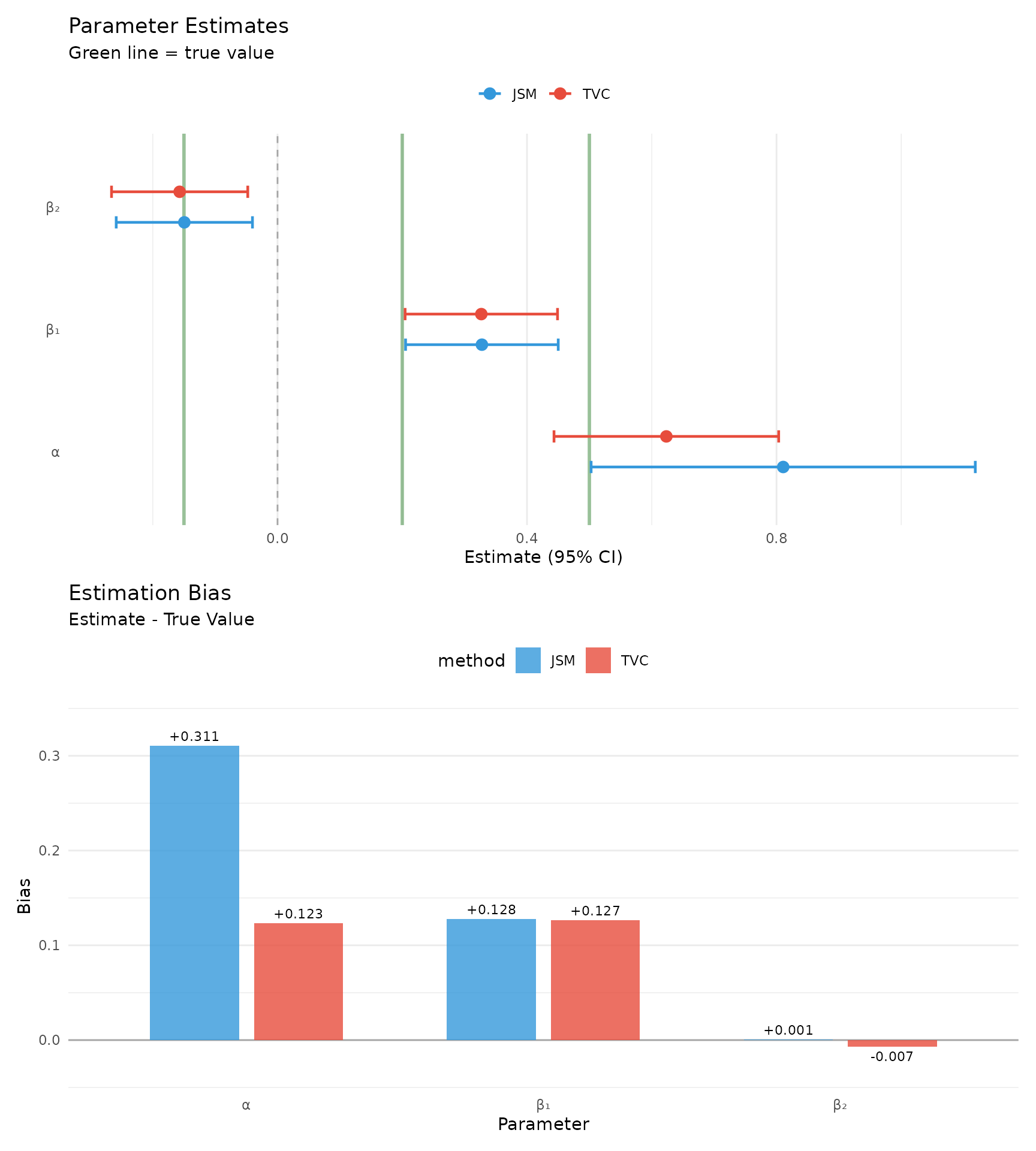
Model Performance
# Calculate C-index for model comparison
library(survival)

# JSM: Combine survival predictors with longitudinal predictions
jsm_risk <- -with(
  jsm_data,
  fit_jsm$coefficients$phi["w1"] * w1 +
    fit_jsm$coefficients$phi["w2"] * w2 +
    fit_jsm$coefficients$alpha * fitted(fit_lme)
)

# Time-varying Cox: Use built-in linear predictor
tvc_risk <- -predict(fit_tvcox, type = "lp")

# Calculate concordance for both models
jsm_conc <- concordance(Surv(start, stop, event) ~ jsm_risk, data = jsm_data)
tvc_conc <- concordance(Surv(start, stop, event) ~ tvc_risk, data = jsm_data)

# Create comparison
cindex_comp <- data.frame(
  Model = c("Joint Model", "Time-Varying Cox"),
  Cindex = c(jsm_conc$concordance, tvc_conc$concordance),
  SE = sqrt(c(jsm_conc$var, tvc_conc$var))
) %>%
  mutate(
    Lower = Cindex - 1.96 * SE,
    Upper = Cindex + 1.96 * SE,
    CI = sprintf("%.3f (%.3f-%.3f)", Cindex, Lower, Upper)
  )

# Display table
knitr::kable(
  select(cindex_comp, Model, `C-index (95% CI)` = CI),
  caption = "Concordance Index: Higher = Better Discrimination",
  align = c("l", "c")
)| Model | C-index (95% CI) |
|---|---|
| Joint Model | 0.619 (0.586-0.653) |
| Time-Varying Cox | 0.640 (0.605-0.674) |
#> R version 4.5.1 (2025-06-13)
#> Platform: x86_64-pc-linux-gnu
#> Running under: Ubuntu 24.04.2 LTS
#>
#> Matrix products: default
#> BLAS:   /usr/lib/x86_64-linux-gnu/openblas-pthread/libblas.so.3
#> LAPACK: /usr/lib/x86_64-linux-gnu/openblas-pthread/libopenblasp-r0.3.26.so;  LAPACK version 3.12.0
#>
#> locale:
#>  [1] LC_CTYPE=C.UTF-8       LC_NUMERIC=C           LC_TIME=C.UTF-8
#>  [4] LC_COLLATE=C.UTF-8     LC_MONETARY=C.UTF-8    LC_MESSAGES=C.UTF-8
#>  [7] LC_PAPER=C.UTF-8       LC_NAME=C              LC_ADDRESS=C
#> [10] LC_TELEPHONE=C         LC_MEASUREMENT=C.UTF-8 LC_IDENTIFICATION=C
#>
#> time zone: UTC
#> tzcode source: system (glibc)
#>
#> attached base packages:
#> [1] splines   stats     graphics  grDevices utils     datasets  methods
#> [8] base
#>
#> other attached packages:
#> [1] patchwork_1.3.2     tidyr_1.3.1         dplyr_1.1.4
#> [4] ggplot2_3.5.2       JSM_1.0.2           survival_3.8-3
#> [7] statmod_1.5.0       nlme_3.1-168        JointODE_0.0.0.9000
#>
#> loaded via a namespace (and not attached):
#>  [1] Matrix_1.7-3       gtable_0.3.6       jsonlite_2.0.0     compiler_4.5.1
#>  [5] tidyselect_1.2.1   Rcpp_1.1.0         simsurv_1.0.0      jquerylib_0.1.4
#>  [9] systemfonts_1.2.3  scales_1.4.0       textshaping_1.0.1  yaml_2.3.10
#> [13] fastmap_1.2.0      lattice_0.22-7     R6_2.6.1           labeling_0.4.3
#> [17] generics_0.1.4     knitr_1.50         tibble_3.3.0       desc_1.4.3
#> [21] bslib_0.9.0        pillar_1.11.0      RColorBrewer_1.1-3 rlang_1.1.6
#> [25] cachem_1.1.0       deSolve_1.40       xfun_0.53          fs_1.6.6
#> [29] sass_0.4.10        cli_3.6.5          mgcv_1.9-3         withr_3.0.2
#> [33] pkgdown_2.1.3      magrittr_2.0.3     digest_0.6.37      grid_4.5.1
#> [37] lifecycle_1.0.4    vctrs_0.6.5        evaluate_1.0.4     glue_1.8.0
#> [41] farver_2.1.2       ragg_1.4.0         purrr_1.1.0        rmarkdown_2.29
#> [45] pkgconfig_2.0.3    tools_4.5.1        htmltools_0.5.8.1