A simulated dataset with 200 subjects generated using the Joint ODE Model framework, demonstrating patient heterogeneity through continuous distributions of dynamics parameters, with longitudinal biomarker measurements and survival outcomes.
Format
A list with two components:
- data
A list containing the simulated data:
- longitudinal_data
Data frame with 17,347 longitudinal measurements from 200 subjects:
id: Patient identifier (1-200)
time: Measurement time
biomarker: True biomarker value (ODE solution)
velocity: First derivative \(dy/dt\)
acceleration: Second derivative \(d^2y/dt^2\)
observed: Observed biomarker with measurement error
x1, x2: Longitudinal covariates (normal distribution)
- survival_data
Data frame with survival outcomes (200 patients):
id: Patient identifier
time: Event or censoring time
status: Event indicator (1=event, 0=censored)
w1, w2: Survival covariates
- state
Matrix (200 x 2) with subject-specific initial states:
biomarker: Initial biomarker value at \(t=0\)
velocity: Initial velocity \(dy/dt\) at \(t=0\)
- random_effects
Matrix (200 x 2) with subject-specific random effects for ODE dynamics:
dyn_value: Random effect for biomarker coefficient
dyn_slope: Random effect for velocity coefficient
Attributes include
mu(population means) andsigma(2x2 covariance matrix).
- init
A list containing initial parameter values:
- coefficients
True parameter values used in simulation:
baseline: B-spline coefficients for log baseline hazard
longitudinal: Fixed effects for ODE dynamics (dyn_const, dyn_value, dyn_slope, covariate effects)
hazard: Association parameters (value, slope) and survival covariate effects
measurement_error_sd: Measurement error SD (0.1)
random_effect_sigma: 2x2 covariance matrix for random effects (dyn_value, dyn_slope)
- configurations
Model configuration:
baseline: B-spline configuration for baseline hazard
gamma: Power parameter for velocity effect (1)
Details
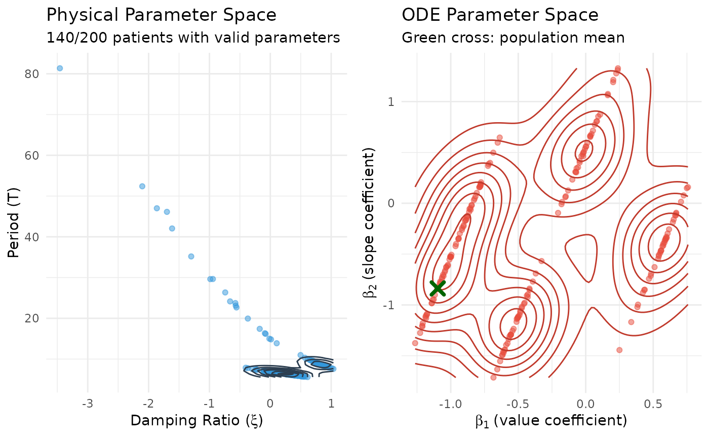
The dataset contains 200 subjects with heterogeneous ODE dynamics. Subject-specific dynamics are characterized by random effects on dyn_value and dyn_slope parameters, which correspond to oscillation frequency and damping in the physical interpretation.
Population-level dynamics parameters:
Damping ratio: \(\xi \approx 0.4\) (mean across subjects)
Period: \(T \approx 6\) (mean across subjects)
These physical parameters are internally transformed to ODE coefficients (dyn_value, dyn_slope) with random effects following a multivariate normal distribution. The init$coefficients provide true population-level parameter values suitable for model initialization and validation.
Examples
# Load the data
data(sim)
# Examine structure
str(sim, max.level = 2)
#> List of 2
#> $ data:List of 5
#> ..$ longitudinal_data :'data.frame': 17350 obs. of 8 variables:
#> ..$ survival_data :'data.frame': 200 obs. of 5 variables:
#> ..$ state : num [1:200, 1:2] -0.27 -0.565 -0.541 -0.573 -0.385 ...
#> .. ..- attr(*, "dimnames")=List of 2
#> ..$ initial_state_mean: Named num [1:2] -0.503 -0.109
#> .. ..- attr(*, "names")= chr [1:2] "m0" "v0"
#> ..$ random_effects : num [1:200, 1:4] 0.2326 -0.0623 -0.0384 -0.0701 0.1178 ...
#> .. ..- attr(*, "dimnames")=List of 2
#> .. ..- attr(*, "mu")= Named num [1:2] -1.097 -0.838
#> .. .. ..- attr(*, "names")= chr [1:2] "dyn_value" "dyn_slope"
#> .. ..- attr(*, "sigma")= num [1:2, 1:2] 0.00134 0.00051 0.00051 0.04406
#> $ init:List of 2
#> ..$ coefficients :List of 6
#> ..$ configurations:List of 4
# Access longitudinal data
head(sim$data$longitudinal_data)
#> id time biomarker velocity acceleration observed x1 x2
#> 1 1 0.0 -0.27026757 0.6429255 1.5460140 -0.444414018 1.370958 -2.000929
#> 2 1 0.1 -0.19856571 0.7878669 1.3525734 -0.067734078 1.370958 -2.000929
#> 3 1 0.2 -0.11333922 0.9134332 1.1588720 -0.106733186 1.370958 -2.000929
#> 4 1 0.3 -0.01652226 1.0197045 0.9670338 0.021566838 1.370958 -2.000929
#> 5 1 0.4 0.08996813 1.1069663 0.7790040 0.009975595 1.370958 -2.000929
#> 6 1 0.5 0.20425317 1.1756901 0.5965405 0.011114903 1.370958 -2.000929
# Summary of survival outcomes
summary(sim$data$survival_data$time)
#> Min. 1st Qu. Median Mean 3rd Qu. Max.
#> 0.9815 8.3783 10.0000 8.6616 10.0000 10.0000
table(sim$data$survival_data$status)
#>
#> 0 1
#> 139 61
# Visualize patient heterogeneity
library(ggplot2)
library(dplyr)
#>
#> Attaching package: ‘dplyr’
#> The following objects are masked from ‘package:stats’:
#>
#> filter, lag
#> The following objects are masked from ‘package:base’:
#>
#> intersect, setdiff, setequal, union
# Examine population-level parameters
cat("Population mean dynamics:\n")
#> Population mean dynamics:
print(sim$init$coefficients$longitudinal)
#> dyn_value dyn_slope dyn_const dyn_x1 dyn_x2
#> -1.0966227 -0.8377580 0.0000000 0.5483114 -0.4934802
cat("\nCovariance matrix:\n")
#>
#> Covariance matrix:
print(sim$init$coefficients$random_effect_sigma)
#> [,1] [,2] [,3] [,4]
#> [1,] 0.010 0.0320 0.0000000000 0.0000000000
#> [2,] 0.032 0.1025 0.0000000000 0.0000000000
#> [3,] 0.000 0.0000 0.0013362015 0.0005103914
#> [4,] 0.000 0.0000 0.0005103914 0.0440598636
# Compute patient-specific xi and period from random effects
# Note: A small number of patients may have invalid dynamics due to
# the tail behavior of the normal approximation
compute_patient_dynamics <- function(dyn_value, dyn_slope) {
omega <- sqrt(-dyn_value)
period <- 2 * pi / omega
xi <- -dyn_slope / (2 * omega)
data.frame(xi = xi, period = period)
}
# Get patient-specific dynamics from random effects
patient_beta <- sweep(
as.matrix(sim$data$random_effects),
2,
sim$init$coefficients$longitudinal,
"+"
)
#> Warning: STATS is longer than the extent of 'dim(x)[MARGIN]'
patient_params <- compute_patient_dynamics(
patient_beta[, 1],
patient_beta[, 2]
)
#> Warning: NaNs produced
patient_params$id <- seq_len(nrow(patient_params))
# Visualize parameter distributions in both spaces side by side
library(gridExtra)
#>
#> Attaching package: ‘gridExtra’
#> The following object is masked from ‘package:dplyr’:
#>
#> combine
# Remove patients with invalid dynamics (NaN/Inf from constraint violations)
patient_params_valid <- patient_params[
is.finite(patient_params$xi) & is.finite(patient_params$period),
]
# Left: Physical parameter space (xi vs period)
p_physical <- ggplot(patient_params_valid, aes(x = xi, y = period)) +
geom_point(alpha = 0.5, color = "#3498DB") +
geom_density_2d(color = "#2C3E50") +
labs(
title = "Physical Parameter Space",
subtitle = sprintf(
"%d/%d patients with valid parameters",
nrow(patient_params_valid),
nrow(patient_params)
),
x = expression("Damping Ratio (" * xi * ")"),
y = "Period (T)"
) +
theme_minimal()
# Right: ODE parameter space (beta1 vs beta2)
beta_df <- data.frame(
beta1 = patient_beta[, 1],
beta2 = patient_beta[, 2]
)
p_ode <- ggplot(beta_df, aes(x = beta1, y = beta2)) +
geom_point(alpha = 0.5, color = "#E74C3C") +
geom_density_2d(color = "#C0392B") +
annotate("point",
x = sim$init$coefficients$longitudinal[1],
y = sim$init$coefficients$longitudinal[2],
color = "darkgreen", size = 3, shape = 4, stroke = 2
) +
labs(
title = "ODE Parameter Space",
subtitle = "Green cross: population mean",
x = expression(beta[1] ~ "(value coefficient)"),
y = expression(beta[2] ~ "(slope coefficient)")
) +
theme_minimal()
# Display side by side
grid.arrange(p_physical, p_ode, ncol = 2)
 # Select example patients across the distribution (only valid ones)
set.seed(123)
example_ids <- sample(
patient_params_valid$id,
min(6, nrow(patient_params_valid))
)
plot_data <- sim$data$longitudinal_data %>%
filter(id %in% example_ids) %>%
left_join(patient_params_valid, by = "id") %>%
mutate(label = sprintf("ID %d (xi=%.2f, T=%.1f)", id, xi, period))
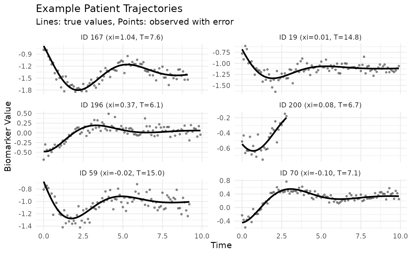
# Plot example trajectories
p2 <- ggplot(plot_data, aes(x = time, y = biomarker)) +
geom_line(linewidth = 1) +
geom_point(aes(y = observed), alpha = 0.4, size = 0.8) +
facet_wrap(~label, scales = "free_y", ncol = 2) +
labs(
title = "Example Patient Trajectories",
subtitle = "Lines: true values, Points: observed with error",
x = "Time",
y = "Biomarker Value"
) +
theme_minimal()
print(p2)
# Select example patients across the distribution (only valid ones)
set.seed(123)
example_ids <- sample(
patient_params_valid$id,
min(6, nrow(patient_params_valid))
)
plot_data <- sim$data$longitudinal_data %>%
filter(id %in% example_ids) %>%
left_join(patient_params_valid, by = "id") %>%
mutate(label = sprintf("ID %d (xi=%.2f, T=%.1f)", id, xi, period))
# Plot example trajectories
p2 <- ggplot(plot_data, aes(x = time, y = biomarker)) +
geom_line(linewidth = 1) +
geom_point(aes(y = observed), alpha = 0.4, size = 0.8) +
facet_wrap(~label, scales = "free_y", ncol = 2) +
labs(
title = "Example Patient Trajectories",
subtitle = "Lines: true values, Points: observed with error",
x = "Time",
y = "Biomarker Value"
) +
theme_minimal()
print(p2)
 if (FALSE) { # \dontrun{
# Fit a Joint ODE model using this data
fit <- JointODE(
longitudinal_formula = observed ~ x1 + x2,
survival_formula = Surv(time, status) ~ w1 + w2,
longitudinal_data = sim$data$longitudinal_data,
survival_data = sim$data$survival_data,
state = as.matrix(sim$data$state)
)
summary(fit)
} # }
if (FALSE) { # \dontrun{
# Fit a Joint ODE model using this data
fit <- JointODE(
longitudinal_formula = observed ~ x1 + x2,
survival_formula = Surv(time, status) ~ w1 + w2,
longitudinal_data = sim$data$longitudinal_data,
survival_data = sim$data$survival_data,
state = as.matrix(sim$data$state)
)
summary(fit)
} # }