Fit Survial Models via Ordinary Differential Equations

Usage

survode(formula, data, df, degree = 3, knots = "uniform", init, control, ...)

Arguments

formula: a formula object, with the response on the left of a ~ operator, and the terms on the right. The response must be a survival object as returned by the Surv function.
data: a data frame in which to interpret the variables named in the formula.
df: the number of degrees of freedom for the spline.
degree: the degree of the spline. Default is 3.
knots: the knots of the spline, either "uniform" or "quantile". For "uniform", the knots are equally spaced between 0 and the maximum observed time. For "quantile", the knots are equally spaced between the quantiles of the observed times. Default is "uniform".
init: a vector of initial values for the parameters. Default initial value is zero for all parameters.
control: Object of class survode_control containing control parameters for the fitting algorithm. Default is survode_control(...).
...: Other arguments passed to survode_control.

Examples

library(simsurv)
library(survode)

# Create a simple data set
set.seed(42)
cov <- data.frame(
  id = 1:400,
  trt = stats::rbinom(400, 1L, 0.5),
  hormon = stats::rnorm(400, 0, 1)
)
dat <- simsurv(
  lambdas = 0.1, gammas = 1.5, betas = c(trt = -0.5, hormon = 1.0),
  x = cov, maxt = 5
)
sim <- merge(cov, dat)

# Fit a Cox model with a spline for the baseline hazard
fit <- survode(Surv(eventtime, status) ~ trt + hormon, data = sim, df = 5)
fit$coefficients$beta
#>        trt     hormon 
#> -0.6693948  0.9394916 

# Predict the baseline hazard at times (0, 5)
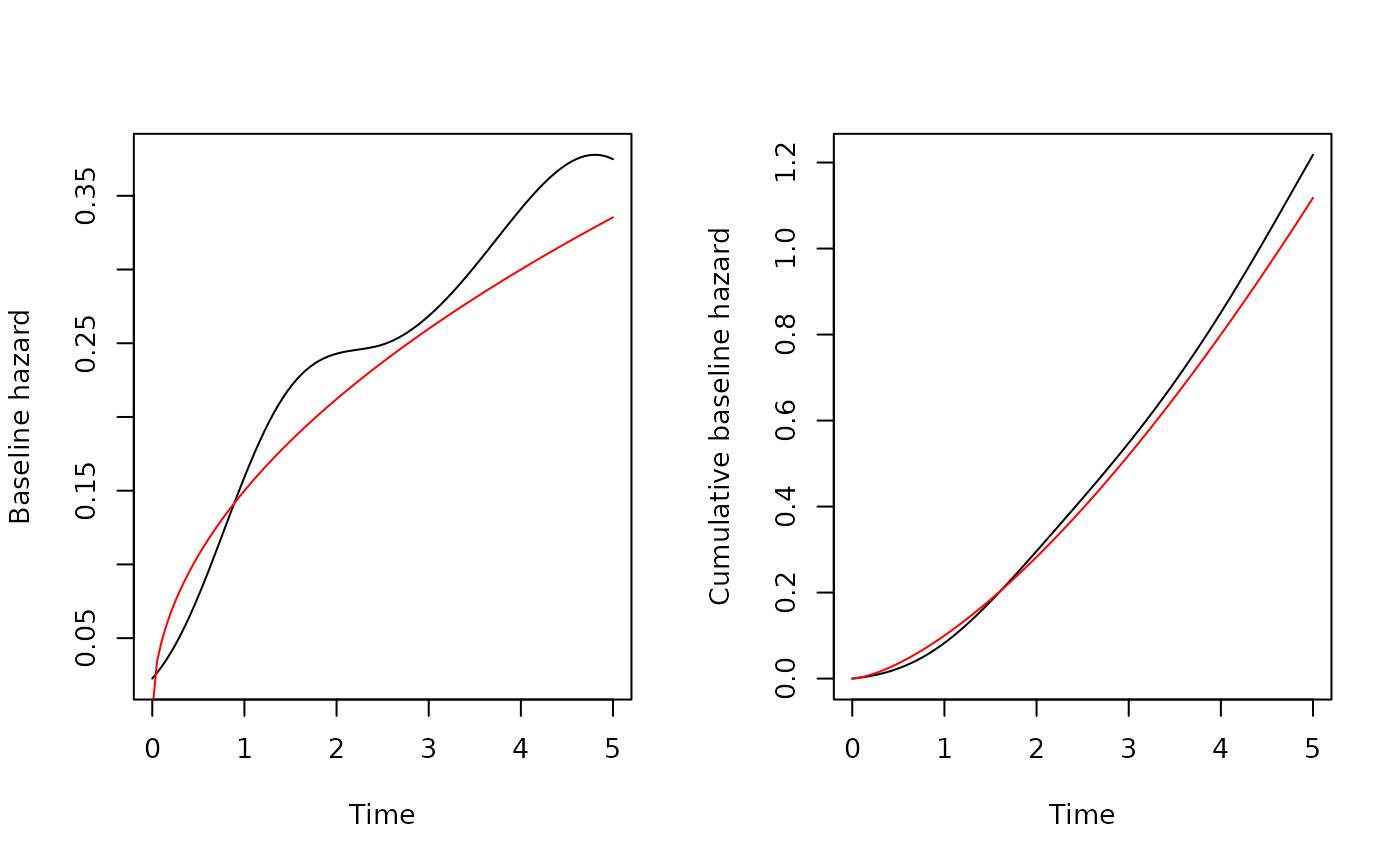
bh <- predict(fit, type = "hazard", time = seq(0, 5, length.out = 100))
par(mfrow = c(1, 2), cex = 0.85)
plot(
  bh$time, bh$basehaz,
  type = "l", xlab = "Time", ylab = "Baseline hazard"
)
lines(bh$time, 0.15 * bh$time^0.5, col = "red")
plot(
  bh$time, bh$cumhaz,
  type = "l", xlab = "Time", ylab = "Cumulative baseline hazard"
)
lines(bh$time, 0.1 * bh$time^1.5, col = "red")